NAM A2: The Team Behind the Technology
We sat down to tell the story of how A2 was built, from activation functions and aliasing to retraining 250K+ models and what may be the largest blind listening test in guitar tone history.
The response has been overwhelming. In just three months, dozens of hardware and software companies have launched NAM A2 and TONE3000 API integrations, and MusicRadar called it an “iPod moment for electric guitar tone.”
We built A2 over Discord and a lot of late nights. Until this video, the four of us hadn’t been in the same room together since A2 launched. With A2 shipped and the first devices running it in front of us, we finally sat down to talk about how it came together.
We go deep into the engineering behind A2, including:
- What are NAM and A2? – Where NAM started and what A2 changes.
- Why A2 was needed – The limitations of A1 and what led to A2.
- Activation functions – Why we moved from tanh to leaky ReLU.
- Dilation pattern and de-gridding – What caused A1’s ringing and how we fixed it.
- The convolutional head – How A2 reduces high-frequency aliasing.
- The receptive field – How A2 captures more time-dependent behavior.
- Slimmable and packed training – How one model runs as A2-Full or A2-Lite.
- Retraining the entire library – How we retrained 250K models from A1 to A2.
- DSP optimization – How we got A2-Lite to 50% CPU on a $3 chip.
- The biggest tone study ever? – 1,000 participants, 100,000+ ratings, and the results.
Watch the full conversation above, or read the transcript below.
Who's in the room
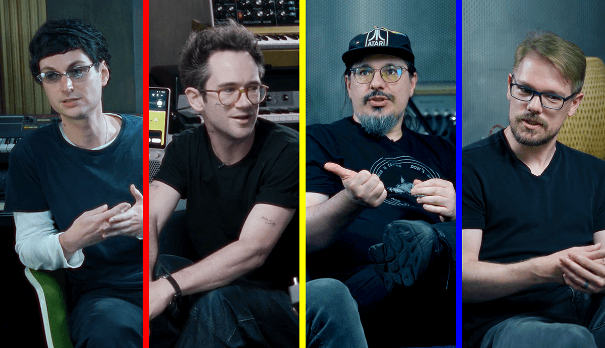
- Stanley Vergilis – Co-Founder and CEO, TONE3000
- Woodbury "Woody" Shortridge – Co-Founder and CTO, TONE3000
- João Santos – Research Scientist, TONE3000
- Steve Atkinson – Creator of Neural Amp Modeler
The following transcript has been edited for length and clarity.
What is NAM, and what is A2?
Stanley: So for those who are unfamiliar — what is Neural Amp Modeler?
Steve: Right. Neural Amp Modeler is an open source project that I created, and it's a way for anyone on this planet to make a model, or a capture, of their guitar or bass amp.
Stanley: And what's A2?
Woody: A2 is why we're all here. It's a project we all did together. It's the new standard for NAM that allows people to create models of their bass amps, guitar amps, pedals and so forth. It's designed to sound way better — more accurate and true to the gear — and, most importantly, to run really efficiently so that it can live on all these devices.
Stanley: For those of you that don't know about TONE3000: TONE3000 is the world's largest community of tones. You can share Neural Amp Modeler captures and you can share impulse responses. You can also create Neural Amp Modeler captures of your own gear on the website — also known as training them. And I think we just hit half a million captures, that have been downloaded 6 million times. So it's been growing really fast.
João, you built a pedal. What does it do?
João: So basically, as we were developing this, we wanted to make sure it was going to run on a variety of devices. On the table there's a bunch of the big stuff, but we had a common minimum platform that we decided on: the Daisy. The Daisy is this tiny board that's distributed as a do-it-yourself music thing. It has a processor in it that's a Cortex-M7. It costs about $3 in volume. It's a tiny little thing.
Stanley: So that's the $3 chip that we've been putting out everywhere.
João: Yeah, exactly. All the pictures of that little thing — that's the Daisy board with the chip in the middle. And that's all in here now.
Stanley: And you built it?
João: Yeah, I built a little circuit board. There are two buffers, one input, one output. And I put an EQ in that's copied from Steve's plugin. It's the same EQ.
Stanley: Should we hear what it sounds like? Should we hear an E chord through it?
Woody: Yeah.
Stanley: Which amp do you have loaded on this?
João: That was a Bogner Überschall, from Amalgam Audio.

Stanley: It's crazy that it's playing on a $3 chip.
João: Yeah. We didn't believe it either. Woody and I did an A/B test — the pedal and the plugin — and it sounds exactly the same.
Woody: That's amazing. This was kind of our North Star throughout the whole process. João had a test bed with this chip.
Steve: Our hope is that everyone out there who's got an R&D team, or engineering, can look at the Daisy Seed and see exactly what the specs are there. It's a fairly familiar spec for people that are doing this kind of engineering. And our hope is that you look at that and see that it looks good — and hopefully that's a green light for building your own products.
Where A2 came from
Stanley: Why don't we talk about the origin of A2, how it started? It would be great to understand what sparked this project. Why did we decide that we wanted to launch A2 and build it together?
Woody: Well, I remember with A1 there was always the push and pull with performance especially. People were coming out with pedals that couldn't run the models, and so they were making distillations that didn't sound as great, and consumers were complaining about that. And then on the accuracy side, everyone — especially when you start to shrink A1 models — was looking for better sounding stuff.
But it all came to a head around NAMM, or leading up to NAMM. There were a few companies that came to us and said, hey, we want NAM on our device.
Stanley: I think it started with Blackstar.
Woody: Yeah. Blackstar was an amazing partner, and they wanted to get it on this speaker here. It has a chip pretty similar to what's in this pedal, a little faster. And so we all came together and said, I think we can do this.
Stanley: And so we called you, and we went to a bar called Casino — which we're all going to be going to tomorrow. And we talked about it, and Steve had the gumption to believe that it was going to happen. And Woody and I were like, let's put together a plan to make it happen together. It was in that moment that it was born.
Woody: Right. It was born over cocktails with Steve.
Steve: And one thing that's worth pointing out about the lead-up, and the decision to try to do this, has to do with: did we know that it was possible? The A1 recipe had been out for several years, I think, before this point. Even though it was really important to me in the meantime to keep A1 the standard WaveNet — to keep that from changing, so that people that wanted to build with this weren't trying to chase a moving target.
I had written a blog post a while back, where there was quite a bit of clamor for a couple of improvements, and I basically said, look, this isn't just my architecture. This is something that many people are depending on, and that makes it a very different situation from how a company might develop a tech that they solely own.
So leading up to A2, there were a lot of technical hints that I was kind of drawing between the lines to say that even though we don't have the exact recipe, I'm seeing hints that it should be feasible to hit what we have in mind. But also, I wanted to make sure that if we're going to do this, we're going to do it for a really good reason, and we're going to make it worthwhile for everyone to accommodate these changes.
Buying gear, and smashing pedals open
Stanley: And a big part of building A2 was involving the ecosystem, involving the industry.
Woody: We had to work for this huge diversity of applications. And in some instances, when people wouldn't respond to our emails, we would literally go to Guitar Center and smash open pedals. Because we hoped that even if you're not responding to our emails, down the road maybe this will work for your company. So we were tearing apart ToneX pedals and different stuff, trying to make sure that what we're building really works for everyone.
João: I remember at a certain point we also made a decision to not lose quality in order to support more stuff.
Woody: Exactly.
João: Because some stuff that's super low cost just doesn't have the compute potential to run a model like this. So we would have to lose a lot in quality. And we were like, no — we want to support a lot of people, but there's a limit here.
Woody: And so through that first phase, that's how we came up with the Daisy as our test bed, on João's side. And then Steve came up with a way to model basically how much compute a potential architecture would take, so that we could plot this stuff.
Stanley: If we're going to talk about how we built A2 — we've peeked into that a bit. We engaged a bunch of hardware partners. And then we bought a bunch of gear.
Woody: That's the best part of the job.
Buying some tube amps. Steve was in Seattle, and then we were here in New York, and both of us were putting together what we had on hand, and going to Guitar Center buying crazy stuff. And the idea was to create eval data. So everything from Mesa Boogies to EVH 5150s. João insisted that we always have —
João: An octave fuzz.
Woody: An octave fuzz.
João: Because they're hard to model.
Stanley: The hardest. What makes them hard to model?
João: It's just their distortion characteristic. It's kind of unpredictable. It's more perceptible if you're playing higher strings.
Stanley: It's like testing the extremes.
João: Yeah. The octave fuzz doesn't care about your signal. It just chops its head off. It's very brutal.
Woody: If you look at the WAV file, it looks nothing like what went in.
But we also used this Ampeg, the vintage B-18 Portaflex. Really, as much as we could get our hands on.
Stanley: I think we had 40 different tones that we tested.
Woody: About 40, yeah. Even outboard stuff — we have some vintage Neves in there that got in there. But the idea was to give us evaluation data, so that as we're iterating on the training recipe, or the model architecture, and what we can fit on these chips, we have a standard data set that we can test how well this stuff is doing.
Finding the juice to squeeze: activation functions
Steve: And, you know, then what places do we have where there's juice to squeeze? One of the things that we found was surprisingly helpful for squeezing out some of that juice was which activation function was used inside the neural network.
So this convolutional neural network that A1 is using had been using a tanh, or hyperbolic tangent, activation function. It's just basically a little S-curve that the signal goes through. And you can really kind of think of it as the neural network doing some saturation on something in the middle. It doesn't necessarily sound like what comes out at the end, but that sort of behavior is probably going to help if you're going to sound like a tube amp.
But machine learning folks have a lot of other options that they might put in place of that little component inside. And so we had a pretty big list of things that we wanted to just check. We weren't just looking at accuracy, which is what a lot of people tend to think about when they're looking at activation functions. But these take a little bit of CPU — and they take a lot of CPU when your neural networks are as small as the ones that Neural Amp Modeler uses. So that's something that we actually didn't see a lot of people discussing in the scientific literature.
But when you factor that in, it turned out that some of these very simple activation functions — the one that actually made it out of our experimentation is called a leaky ReLU. It's basically just got, like, one little kink in the middle, and it's just two kind of straight lines before and after. It's very simple to compute, which means that it takes very little CPU. And we were able to use that CPU basically in other parts of the neural network to improve the overall performance.
A New Activation Function
A1 used Tanh as its activation: accurate, but expensive on small networks. A2 switches to leaky ReLU, which costs less CPU. Those savings went into a larger network that is more accurate at the same CPU budget.
Stanley: Got it. And the activation function in A1 was tanh. So having the lighter activation function gave you guys the ability to create a deeper network with less CPU, so it can be more accurate. Is that right?
Woody: Yeah. It's kind of counterintuitive, because tanh is a full curve, more accurate, versus leaky ReLU, which is just a couple of comparisons. But at our scale, putting those resources into making the network deeper gives you more accuracy.
Before we even started playing around with activation functions and the dilations and all that, though, we did some benchmark modeling. With everything that we recorded, we made A1 models — the standard, the Nano. We went out and bought Neural DSP and ToneX and everything that has a similar goal. We don't know exactly what they're doing inside, but our thought was they're trying to reach the same goal. So let's make sure that we're benchmarking against everything that's available.
Tens of thousands of trainings
Stanley: And then we ran like 10,000 HPO trainings. Can we talk about what that process is, what that means?
Woody: Well, this morning I woke up — and I know we've been throwing around the number 10,000, because we just knew it was more than 10,000. But on our cloud runs, I ran a little script, and I think it's closer to like 15,000. And then on my personal computer there was like 5,000 there.
Stanley: Call it 20.
Steve: Yeah, I've got a tranche of them on my desktop.
Woody: And João probably has a ton.
João: Quite a few, too.
Woody: So yeah, I think tens of thousands of models were trained.
Stanley: And talk about the process, and what that means.
Woody: The purpose is to figure out an architecture, or a recipe if you're talking about training. And to do that, you come up with hypotheses, or you sweep something that you have to play with. And we did a ton of that. Similar to the activation functions, we tested — I don't know, every single one.
João: Probably a dozen.
Woody: A dozen, yeah.
Stanley: So basically, you're tweaking the recipe for what A2 could be, and then running zillions of tests and comparing how these new models that you're tweaking compare to the commercial modelers and also A1. Is that right?
João: Yeah. With the constraint that, of course, if you're doing a sweep, you could look at the biggest models that use the most CPU and go, those are the winners. But that's not what we wanted.
Stanley: The goal was to do exactly the opposite.
João: Yeah. We had a constraint. So it's like, which models live in this region?
Steve: We used a variety of specialty methods to kind of explore little sub-problems along the way. We weren't just letting a computer run, spending an AWS bill without any supervision. For months we were in the weeds, kind of looking closely at these promising things, trying to figure out: okay, which parts of this do we keep, what parts do we kind of look around to see if there's something close by?
João: I think something super important to bring up here is that in traditional HPO, you're usually optimizing a mathematical function, so you just have a number you want to minimize. In this case it was not just a number we were minimizing — Steve was actually listening to models. So he was part of the cost function.
Woody: Exactly.
João: And that's why we needed a mechanism to steer, because we couldn't just rely on, oh, the loss is lower, this model is good. That's not how it works.
Woody: Yeah. There was that angle, the human in the loop. And then also we were modeling: is this going to fit within the CPU budget? But at the end of the day, your test bed was in the loop too. So as we came up with candidates, then it was off to João to see.
Stanley: The test bed was to evaluate the CPU cost of the models.
João: Yeah. So they would send me a bunch of models, and it would be like, oh, this one takes 70% of the CPU, this one takes 60, or whatever.
Dilations, ringing, and de-gridding
Stanley: So now that we're talking about how A2 works, maybe we can jump to the dilation pattern and de-gridding. I'd love to hear a little bit about how that works.
Steve: So folks who have looked into some of the A2 files will notice that part of the architecture is this dilation pattern. If you look at A1, you'll see these very nice powers of two: one, two, four, eight, 16. What this is accomplishing is it's having the convolutional layers kind of gather in data from different amounts of time into the past, to make the prediction. And it happens that if you organize them in that nice geometric sequence, it's very easy to tell exactly how much data that you're pulling forward. We know that a tube amp kind of has a little bit of a history dependence on it. So it seems like a very reasonable thing to do.
The A2 Dilation Pattern
All 23 layers of A2. Three dilation stacks share a hand-tuned, non-doubling schedule (1, 3, 7, 17, 41, 101, 239). Between stacks two and three, wide-kernel degridding layers fill in the gaps, possible because A2 mixes kernel sizes in one layer array.
But after having A1 out for such a long time, we had noticed some comments about kind of unpleasant frequencies that would pop up here and there. And sure enough, as we were looking at some of the quantitative metrics like ESR, sometimes there would be these models that got a really good number — but when you listen to them, there would be this odd ringing sound to them.
So we did a little bit of puzzling about that, and I basically came up with a hypothesis that this was related to what those dilations were, and to the patterns in how the signal is traveling from those past samples through the network into that prediction of what's happening right now.
It turns out that you can somewhat predict where the trouble frequencies might be based on that connection pattern. We'll have more details to say about this when it's all written down. But we basically had a crude idea, or a model, of that, and we used that to sort of steer what specific numbers we were choosing, so that we could anticipate that these artifacts would be largely suppressed.
Woody: Yeah. João made a meta-RNN in like two days.
João: Yeah. We ran an RNN, and we were interested in Wiener-Hammerstein. We were trying a bunch of stuff at that point.
Woody: It kind of shows how many stones we turned over. Not only within the A1 architecture, trying different stuff out, but also looking wider.
Stanley: And talk to me about the gridding, and what problem that was.
Woody: So it kind of goes off of what Steve was saying. To sample the history, it's not sample by sample, it's this pattern. And the reason we do that is it would be too much computation to literally look at every sample. But when you do that — even when you come up with super cool magic numbers like Steve did — you can still wind up with this kind of gridding thing, where you're getting too much of the same kind of frequency, and you may have holes where you're missing out on data, if that pattern is being repeated. And that was leading to the ringing that we were hearing.
So we spent a ton of time on that. There are two layers with a larger kernel, and kind of odd numbers that don't show up in the pattern, and that can kind of be thought of as a de-gridding step. It's kind of this weird, like, local remix. I was thinking about it this morning in terms of presenting it to musicians: it's like you're writing a song, and then you have a bridge in a completely different time signature, and then when you go back to the chorus it's no longer on the Pro Tools grid. That's basically what we did.
Spectral Ring Artifacts
White noise bursts run through each model variant. Pay attention to the ringing artifact around 10 kHz.
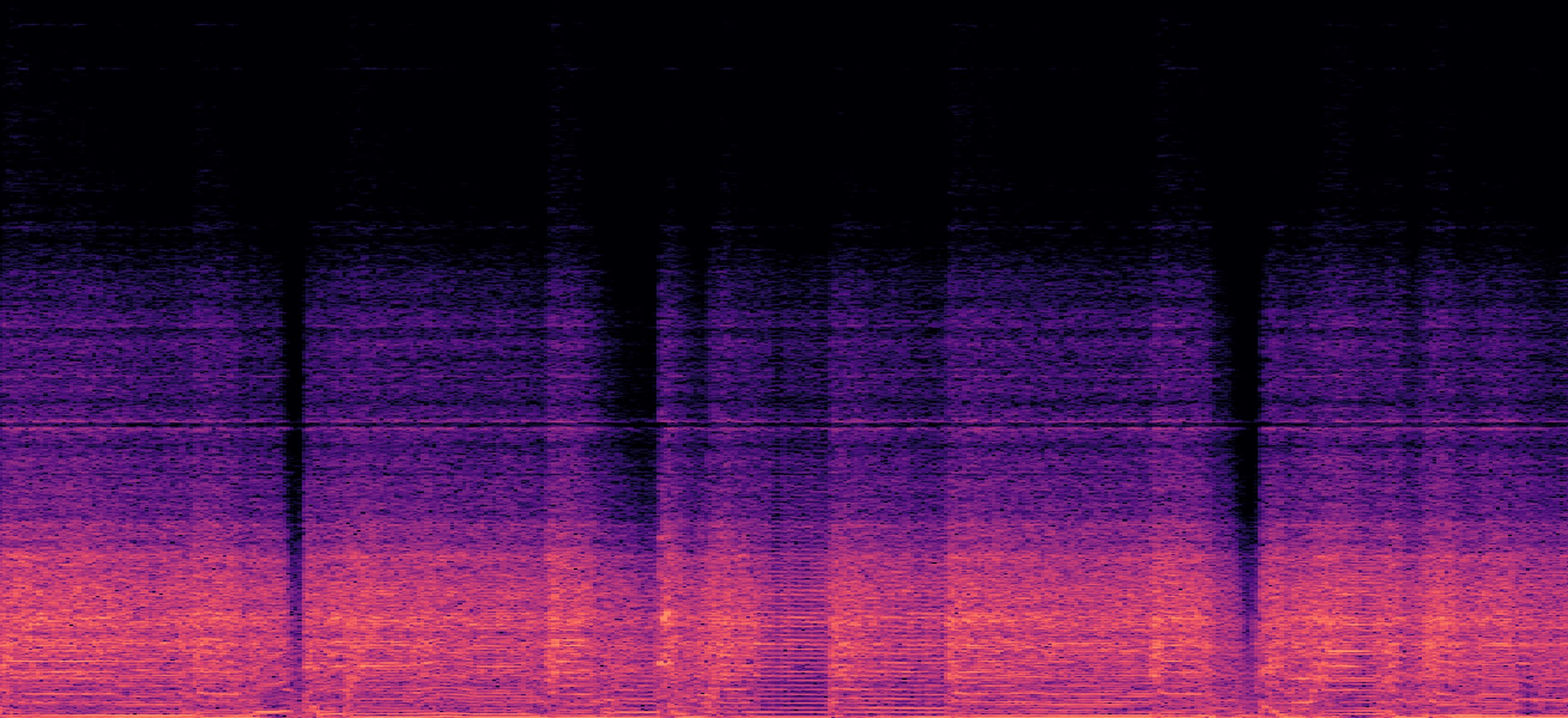
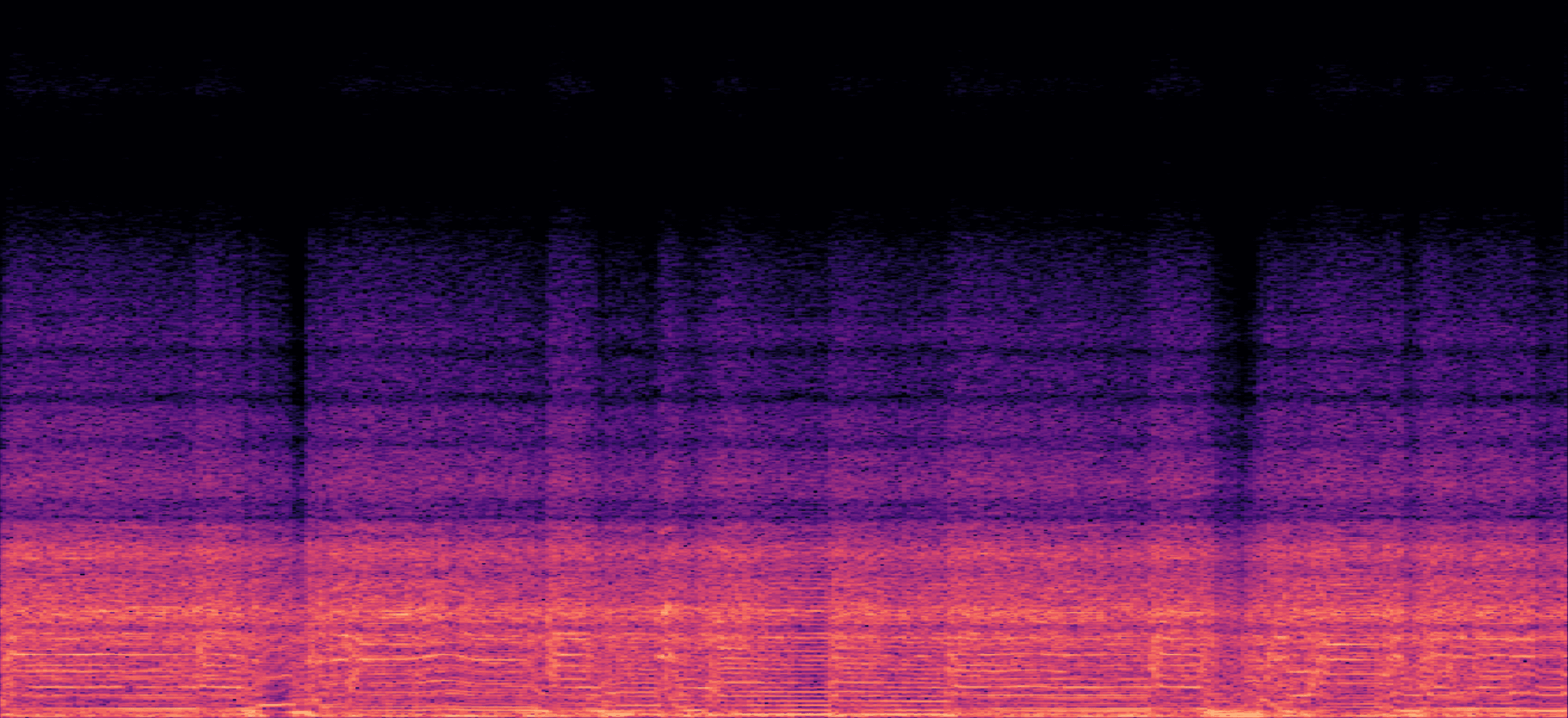
So now you're sampling stuff that shouldn't be repeated, essentially.
Stanley: And that was a huge project of ours, because we had this metallic ringing when we were testing for Blackstar. I remember being in the studio here with Woody at like four in the morning, bleary eyed, had a few beers, and we were like, what are we gonna do about this ringing? But now the models sound great.
João: And the thing is, we reached the conclusion that we could predict these things later — because at first it was just us changing things and going, oh, the ringing frequency changed. Oh, why is it not there anymore?
Steve: I remember I was really excited about it. And actually that's worth — that bears repeating here — a lot of these models did sound really good a lot of the time. But there would be just this one case here or there, and we just couldn't let it go.
Stanley: And that was our job. Our job was to listen to zillions of models and look for tiny artifacts that most people wouldn't be able to tell — because if you have an amp in the room that you know, and you know the tone of, and then you try to capture that, you can tell the difference.
João: And we need one recipe that works for everything. We can't have: oh no, you're modeling a fuzz pedal, you need to use this one. Oh, you have more gain than such and such. No, that doesn't work.
Woody: To Steve's point too, it was like — especially with ringing and different artifacts like that — it could be that we trained the same architecture with the same training data, and ten times it sounds great, and then on the 11th there was an artifact. And we couldn't settle for that, because at TONE3000 scale we're doing hundreds of thousands of models. It has to be consistently great all the time.
The convolutional head, and aliasing
Stanley: Talk to me about the convolutional head. What is it?
Woody: Yeah. So just another kind of cool call-out of the architecture. Basically all the computation of the network, at the very end, turns into audio, right? So that all gets mixed together. And in the original architecture, that was just sample by sample. And what we ended up doing is giving it a little bit of a window, so it could learn how to mix better, to be more accurate.
And the striking thing that we found was the high frequencies. If you look at a spectrogram of A1, after like 15,000 it starts to get pretty crazy, and it doesn't look anything like the original.
Stanley: Aliasing.
Woody: Yeah, but also just high frequency in general. And then with the new architecture, the difference is striking. It follows the true nature of the amp to a T, all the way up.
Stanley: I remember looking at those graphs.
Frequency Response vs the Real Amp
The measured magnitude response of a real amp, compared against its A2 and A1 captures. A2 tracks the full band. A1 stays close, then diverges in the top.
Woody: And so not only does it help us model the high frequency better, it seems, but it does help with aliasing as well — because inherently the higher frequencies are what could cause aliasing-like artifacts.
Stanley: And aliasing was, at least in the hardcore part of the NAM community, something that people were really excited about potentially fixing with A2. How do you feel about the results?
Steve: Don't worry, the silence gets edited out.
João: Stand by for 20 minutes.
Steve: Don't worry. I've got a whole 30 seconds.
Stanley: I mean, there was an improvement. It was a massive improvement.
Steve: Yeah. So when it comes to questions about aliasing, or these kind of specific artifacts that you can pick out of any sort, we're obviously using our ears as the final gate to just tell us whether or not we've done something that sounds good. And I've said this in the past: if the numbers look good and your ears don't like it, then the numbers are wrong.
So in terms of this convolutional head — this is just basically a layer that collects a little bit more of the calculations that the rest of the network had done, as one final pass to make its prediction at the end. And what we had done is we gave it the ability to look at several samples of predictions. It looks a lot like having an IR at the end of it. It's a little different, but it's a very short one as well. And so what that means is that it's going to have exclusive control over high frequency content. And coming back to the way that it sounds, I'm really pleased personally with the way that the high frequency content and details came out.
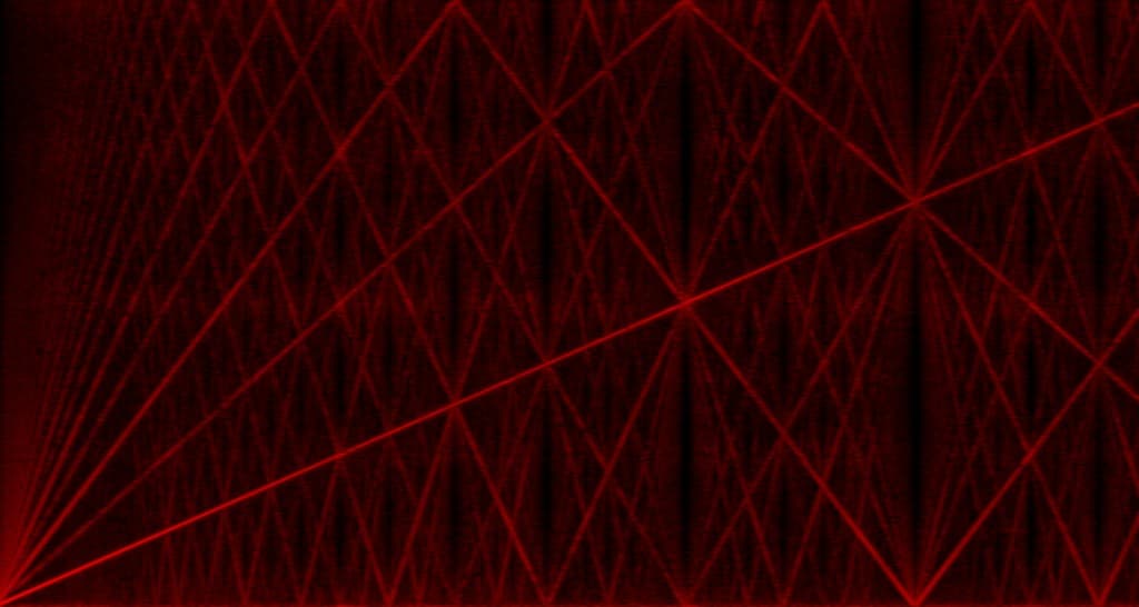
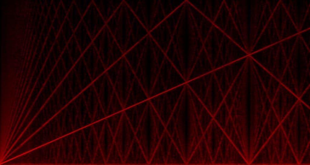
Stanley: You can tell. There's a huge difference. When we were testing for aliasing by bending high strings, you could hear these like weird lower harmonics. The difference between A1 and A2 is night and day. And we were working on this with Blackstar, and they were very excited by the progress that we made. I remember it being a massive achievement.
Aliasing-like Artifacts
Sine sweeps run through the old and new model designs. Full chirp is the full spectrum, unfiltered. Band-passed zooms in on low-frequency inharmonics the model invented (absent from the recording).
João: I'd never even thought of that — some of the tricks to listen for the artifacts they were looking for.
Steve: Let's not tell anyone out there what they are.
João: They'll start looking for them.
Woody: We tried a lot in terms of these aliasing-like artifacts. And João made this really cool tool that came up with metrics, and we could run different ideas by it. And a lot of what we tried was actually on the training side — these loss functions that penalized inharmonics, or different stuff like that. But what I'm really proud of is that we were able to solve it in the actual architecture.
João: With generic improvements.
Woody: Not playing whack-a-mole after a model.
How much history matters: the receptive field
Steve: So like I mentioned this just a little bit earlier, but just to repeat it: a guitar amp, it'll distort your signal. And a lot of people's first thought of distortion is this thing that just takes each sample and kind of bends it in an S-curve. The reality with a tube amp is a bit more subtle. People describe things like sag, and bias, and compression — these things that basically mean that what's happening right now depends on what just had happened a little bit before.
For a tube amp, you can maybe run an impulse through it, kind of see how long it takes that to die down, and get something of an estimate of how much history matters if you want to accurately predict how a tube amp sounds. I came up with something around a tenth of a second. And so you'll see that in A1, its receptive field is about 4,000 samples, at the 48,000 samples per second that it's processing the audio.
As we were messing with those dilations that we talked about earlier, that changes what the receptive field is. And so that kind of opened it up as something that we could, first of all, keep an eye on. We want to make sure that we are staying within a ballpark that is going to reasonably be able to predict what an amp is doing for the right reasons, because it can see everything that matters.
But we tried a few alternatives. We tried combinations of dilations that would get short receptive fields, ones kind of closer to A1, some that were far larger — and basically took metrics, listened to them, kept an eye on how frequently they would succeed at training. Some of them would do really well, but very infrequently.
What we ended up with was something that is pretty close to what A1 had. If I recall correctly, is it something around 5,000 and change samples?
Woody: I don't know the sample number, but I think it's actually quite a bit longer. It is bigger. I think when you convert it to milliseconds, A1 was like 84, and then A2 is like 132. Quite a bit bigger.
Steve: I did remember that it was, in my mind, a little bit bigger. As with a lot of the stuff that we were checking as we were iterating on the design, the thing that reigns supreme is the metrics — whether those are quantitative, or whether they are subjective, us listening to them. We did find that longer receptive fields just tended to give us results that we were more happy with.
A constraint that does start coming into focus, though — especially for some of the pedals that are using these really affordable chips inside — is that you have to hold on to all of that data from the past in order to be able to predict with it. That's bytes and kilobytes, and not megabytes, I don't think, for this.
João: No. But yeah, when you start looking at a pedal like this, it has like two megabytes of memory. And half of it is slow. So it starts becoming a constraint.
Steve: Yeah. So practically, as we were looking at all these things, there's another constraint: it has to fit on the memory on the chip that is going to be able to be communicated with quickly. So it was kind of a few things coming together. The dilations, the receptive field — and I'm really happy with the combination that we came up with.
That's one of the things that I think got most of the training and experimentation. It's like, which sequence of numbers is the right sequence? So trying to get through that as quickly as possible, because there's a lot of sequences of numbers out there.
Woody: There are a lot. With the receptive field, we were going after our eval data set, the 40 tones that we recorded. And that's what we were doing HPO against, finding what works and what doesn't. So that was really for amps, tube amps, pedals like fuzz pedals, and outboard gear. Enlarging the receptive field was to that aim.
But I will say, now that A2 is done, I've been playing around with captures for verified profiles that are going on TONE3000. And it's really fun to hear people doing compression pedals.
Stanley: You're noticing a difference?
Woody: Huge difference from A1. And also, like, room mics — just the reflections in the room from a full rig profile that's done with, like, a ribbon mic.
Stanley: Just capturing more of that time-dependent behavior.
Woody: Exactly.
One file, two sizes: slimmable models and packed training
Stanley: So for those that don't know, training is obviously capturing a NAM profile, or creating a NAM profile. And there was a very special part of A2, which was slimmable, which obviously did not exist in A1. So maybe we could define: what is slimmable training?
Steve: Right. So A2 is slimmable, and what that means is that you'll get one model and you can use it multiple ways. We've got all of these different products. They are running different chips inside.
Stanley: Different processing capabilities.
Steve: People have very different laptops and desktops from each other. They have Raspberry Pis and all these sorts of things. I wanted to be able to truncate, or slim, the neural network, so that people could pick that kind of trade-off between compute and accuracy that works for their needs.
Stanley: Yep. And so one A2 file can be run as A2-Full, which is for pro audio and devices that have enough processing on them. And then that same file can also be run as A2-Lite, which is the size that's designed for embedded hardware that doesn't have as much processing.
So why don't we talk about training?
Steve: Right. So in order to train one of these slim models, there's an infinite number of ways that you could do it. Despite all of the variety in platforms that people were building with, we noticed certain patterns, and it looked like if we kind of built these two well-tailored sizes — and we actually kind of developed them at various points separately — that if we could make both of those work at the same time in one slimmable model, then that would be all that we'd need.
Stanley: Yeah. Especially if A2-Lite sounded good, which it ended up being incredibly accurate.
Steve: So I did basically another revision on how to train a slimmable model. I call it packed training. It is still a method where you are kind of training these two models together at the same time, and it is more efficient than doing one and then doing the other, and then just squeezing them together at the end. That was really important. I didn't want to have us going around and just, like, training a whole grocery list of models. Every time someone asked for one model, it had to be really worth it to get both of them at the same time.
Stanley: Got it.
Woody: I think with packed training — because we figured out with the computation requirements that really we're looking at two different sizes that we needed to make — that allowed us to do packed training where we're not compromising on the accuracy. Because inherently, with the slimmable paper that you put out, it's different sizes trying to solve two different goals. It's trying to sound good being big and sound good being small at the same time. Versus packed, where the two sizes are kind of separate.
Retraining the entire library
Stanley: And maybe João and Woody, you can talk to me a little bit about the retraining process. Obviously TONE3000 has hundreds of thousands of models, and all of those models were A1 — some of them were custom architectures and some of them were other architectures. And so we had this mammoth project of retraining the entire library so that users wouldn't have to go do that themselves. Maybe you could talk us through a little bit what that looked like.
Woody: Yeah, well, it was the whole team. First we had to come up with the training recipe. And similar to how we made the models, same thing: training thousands of models, trying different loss functions. We again just threw everything at it that we could.
You wouldn't know it looking at the training recipe right now, because it's really simple, which is beautiful. It's like, we tried so many different schedulers. We tried weird auxiliary losses. We tried different weights to everything. And in the end we came up with something really simple, and that's what we went with — for what people are now training as they go, and also what we went with for the retraining of the entire library, which I think João should talk about, because he's a madman.
Watch Leaky ReLU Learn a High-Gain Amp
A tiny neural network with leaky ReLU activations, training live in your browser. The gray line is a high-gain amp's output; the yellow line is the network's prediction. It starts as noise and learns the amp's response through gradient descent, the same process that trains a NAM capture.
João: Yeah. So, how many models did we retrain? Like 250,000, something in that range.
Woody: Yeah, and it's still going on. It's still going as we're talking. There's a cluster of H100s.
João: Yeah. So basically I asked Woody to give me a list of all the models on the website ranked by popularity, so we could train the more downloaded ones first. And the other thing we needed to figure out was how to do this efficiently — because if you haven't checked the costs for cloud computing for training AI models, they're huge.
Stanley: I know I don't check.
João: Make sure your money's well spent.
Stanley: Our money.
João: Yeah. We also had to do it quickly, and with the resources that were available.
So, the way models are trained on the website right now, it's on demand: you get a request, that model gets trained as fast as possible, delivered to the user. In this case, because we could afford to wait a little bit — but we still wanted it to be fast — we tried to maximize how much we were using from each GPU. So instead of training one model at a time, we tried to fit as many models as we could in a single GPU. And that varies depending on the GPU, because our farm was a little —
Woody: Heterogeneous.
João: Heterogeneous, yes. So some GPUs were huge and we could fit like 64 models. And some were small and we could fit like 16.
So basically we have these huge jobs submitting thousands of models to these cloud providers, and then they get trained and saved to the cloud. And then I tell Woody to sync, and then they get uploaded to the website. And there's no change whatsoever in the recipe or the result — training models in this way is exactly the same as training them individually. It's just way more efficient and cost efficient for us. So everyone wins.
Woody: I think throughout the process, we were running error metrics against our eval set, right? And we did the listening testing on that eval set, which I'm sure we'll get into. But when we started doing the retraining, that was really gratifying, because at that point this was tone data that we had never tested against before. And all of a sudden we could look at 100,000 retrainings — retraining the models that were trained as A1 — and say, apples to apples, how does this compare? And hopefully we can throw up a chart.
João: Up to this point, we were always looking at those 40 models. Now we could look at statistics and see how many models perform better, like, more accurate.
Stanley: And what we found was that A2 compared to A1, we were seeing about half the ESR. Is that right?
Woody: Yeah. When you control for other variables and look at a standard-to-A2 pool, absolutely.
A2 vs A1 Accuracy
We retrained the entire library of A1 models with A2 and compared the resulting ESR against the original A1 captures (lower is better).
João: There's some models that are a little different because, as you said, there are custom models, there are models that were trained for longer in the past. And now we use the same recipe for everything, because that's just how we want to try to do things.
Stanley: And a question that's come up in the community is, how did we retrain the models that we didn't have the training data for — where somebody trained off of TONE3000 and they uploaded their model to TONE3000? What was the process there?
Woody: Yeah. So there was a good amount of data wrangling to make sure nobody was left behind. The idea being that if all of these devices update their firmware to support A2, we don't want your old A1 models to not work. So even for models that people had trained locally, what we did is we rendered synthetic training data through the old models and retrained on that synthetic data.
Stanley: So what does that mean? You're running a sweep signal through the A1 model.
Woody: And then training on that. And it's really just a compatibility step that takes an A1 model and makes it A2 compliant, so that it can run as A2-Full or A2-Lite.
And then we also had people who had made these dry/wet models. That took a bit of data pre-processing and some guessing.
João: One requisite to train a bunch of models at the same time is that all the training signals are the same duration. And with dry/wet —
Stanley: I remember seeing a lot of Discord messages about this.
João: With dry/wet they're often not, because each person will record however long they want. So we normalized it. We made a bunch of buckets, like, different lengths. That means we had to trim some of them. But in the end, most of them sound either as good or better, so there's no complaints.
Making it fast: the DSP work
Stanley: Amazing. So we've talked a lot about how A2 works, the architecture, the retraining process. Now, a massive effort and goal of A2 was for it to run on these processing-constrained devices. So João, you were an absolute monster in this domain. Talk us through the DSP optimizations, what your process was. This is your moment.
João: All right. There's a lot to talk about, but I'll try to be brief.
So basically, the code that Steve had open sourced before was reference code, and it was mostly tested as a plugin. It worked really well on desktop. It was doing what we needed to do. But now, at this moment, because we needed to run on constrained devices, it was very important to go and evaluate each block of the model. And we already had a good idea for that, because we had run all these tests to see, like, oh, how much does a convolution cost?
And a lot of it is related to how the architecture is. In these smaller, more constrained computing devices, they don't do a thing that desktops do that's called vectorization. So they have to do one operation at a time, more or less. They can do tricks, and they also have different constrained memory layouts.
So we had to basically look at a bunch of stuff. Once we identified what was taking too long, we looked at the code and were like, oh, what's being done here? How can we optimize this? Like, trying to do just this operation — if I change this, is it faster? And we did that several times. I published them on GitHub — I think there's like 17 different micro-benchmarks. And for each of them we were like, can we make this faster? And whenever we saw we could make it faster, we shipped it.
And then at the end, we ended up adding it to NAM Core, in what we call A2-Fast. That's a collection of all the tricks we found to make A2 run faster. And that's not only these single-operation things, but there are also all these operations that are happening that mean we have to process some data, save it somewhere, and then we go back and look at it and we process it and save it again. And now we're kind of streamlining it, so you can do a bunch of stuff in one pass on the Daisy.
So for A2-Lite, we went from not being able to run it at all to only using 60% of the CPU. So it was a big deal.
Embedded Inference Speed
Whether A2-Lite can run in real time directly on resource-constrained embedded hardware.
Woody: The first time I think we handed this off to João to give us a benchmark, I think the response was, there is no way.
João: No way.
Woody: And then we said, try a little harder.
João: Woody says I have this habit of —
Woody: João under-promises and over-delivers.
João: So it's like, I'm not sure I can make it 30% faster. And then I'm like, I made it eight times faster.
Stanley: There were a lot of, like, mind-blown emojis when João was delivering the results in Discord.
João: And I think one really nice thing is that some of these tricks we learned also work for A1. So we also made A1 faster. So there's not only the things we changed in the architecture that make it more efficient, like the activation function, but also how we compute things in a more streamlined, optimized way has a lot to do with it. Especially on the Daisy, it has a lot to do with, like, are we using the right type of memory? Some memory is faster than others, that kind of stuff.
Woody: You should be able to just grab what he did and implement it. Maybe make your own tweaks for your specific platform. But it just adds to the kind of open source toolset that Steve originally started. There's a lot more for people to grab now.
João: Yeah, we don't want to keep those tricks for ourselves.
I think one thing that is important to just bring up is that a lot of the optimization at first was focused on the Daisy, because it's a particularly difficult platform to work with. And then on desktop. Because those were the extremes. And now we're working with partners who make these amazing pedals.
The numbers
Stanley: Should we talk about the results?
João: Yeah. I think for CPU performance, for constrained platforms: we went from A1, where you couldn't run A1 — there was no way you could run A1 on a chip like the one in the Daisy — and now we have a model that performs really well and can run on that chip. We are allowing partners to run A2 on a variety of pedals. And because they use less compute, that means you can run more stuff. Like, you can run more effects, or you can run multiple NAMs. Steve made a fun experiment in his video where he put, like, 100.
Stanley: What were the numbers for A1 standard versus A2-Full on — I think you had an M1?
Steve: Yeah. So this is a cute experiment that I did with my MacBook. Before I say these numbers, it's probably worth saying that this is not how we usually benchmark these models.
Stanley: This is infotainment.
Steve: Yeah, well, this is for entertainment. So I've got a MacBook Pro that is, I think, six years old.
Stanley: The M1.
Steve: Right. It's still the new Apple silicon; it's not so old that it's Intel. But I figured that it would be kind of illustrative to just pull up as many plugins as possible, each just running a NAM model at a time. I did try it with A1 as well, just to kind of get a point of comparison and a sanity check. The numbers, as I remember them — because they are memorable — is 46 A1 standards, 64 A2-Fulls.
Stanley: Which is 30 to 40%.
Steve: Which is basically in line with what the real-time-factor, model-only results were suggesting. I've got details that I state in the video that I put out about this. But with the small models, A1 Nano, I think, was somewhere a little north of 100, and A2-Lite —
Desktop Inference Speed
How fast A2-Lite runs on a modern desktop CPU, and how much headroom is left for the rest of your signal chain.
Stanley: Which sounds way better.
Steve: Yeah. It's worth repeating how much better A2-Lite sounds than any small A1 that we had in the past.
Stanley: A1 standard to A2-Full: 30 to 40% improvement in CPU cost for A2. I guess what that means is, for two A1 standards you can run three A2-Fulls. And the A2-Lite can run at 50% on the Arm Cortex that we've been benchmarking. So that's a pretty insane accomplishment.
A1 vs A2 Inference Speed
How the new A2 models compare to the original A1 architecture on the same hardware.
Woody: And all these benchmarks are before João's latest PR.
João: There's a later one. It will get a little faster — 20% faster. It's only for larger models.
Woody: We were talking to the Darkglass people about this one.
João: On that pedal, we made it run twice as fast.
Stanley: And in the past couple of days? This is why I called you a monster. Speed demon.
Steve: One thing to wedge in there as well on the CPU discussion is that, as we were saying, even though we released A2, CPU optimizations are still possible.
Stanley: Still happening.
Steve: This was actually something that was happening during the development. We were fighting on these little trade-offs, and then all of a sudden João would figure out how to make everything run a little bit more quickly, and then all of a sudden the options would open up a little bit.
Woody: We'd make the network a little bit bigger.
Steve: Which is maybe one of the things worth pointing out — why it took us a little bit longer than we had originally sort of quoted. We had this kind of sequence of things getting better, right? And there were a few points there where we realized that it looks like we may be able to really substantially improve what we're going to deliver. And as we were thinking about this — we want to make this last — we basically made the decision that we're going to wait a little bit longer, we're going to see this through and really make A2 better. And frankly, I'm just really thrilled with where those experimentations and side quests landed.
The listening test
Stanley: Let's talk about the accuracy, the way it sounds. That's why we're all here, after all. Pun intended, I guess. How do we feel about the results?
Steve: So, the quantitative tests: a variety of numbers that we're keeping an eye on, because we think that they kind of correspond to how good the method is working. So folks that have been following NAM things in the past will be familiar with ESR — error-to-signal ratio.
This is basically a lower-is-better number. When it's zero, there is no error, no difference between the model and the tube amp that you recorded. Lower should be better — but that's why we have a few other numbers to sort of check against that.
So we have a frequency domain — or a couple of different frequency domain losses, or metrics, that we were looking at. One of them that's been around is this multi-resolution short-time Fourier transform loss. You basically can think of it as: in time, in frequency, you can kind of see a heat map of where the sound is. I'm just thinking about, like, folks that do birding — apparently they show these spectrograms, they can kind of see what the bird sounds like. This is kind of the same thing. You can see what the amp sounds like.
You can put the same thing on top for the model. If it's wrong, because there's a ringing frequency, or because these frequencies are aliasing downward, those are differences, and it penalizes the number. It goes up, and down is better. We have a version of it where we were looking at it on a small scale, more closely, that kind of groups the frequencies in the way that we kind of hear them.
Stanley: And what would we see for A2-Full and A2-Lite?
Steve: I don't remember the exact numbers, but we definitely saw results that made us say, that's what we were going for.
Stanley: Yeah. So I think A2-Full beat A1 standard, Line 6, IK Multimedia's ToneX and Neural DSP by a wide margin. And then we also saw that A2-Lite beat them as well, with A1 standard and A2-Lite being pretty close quantitatively — but especially in the listening test. So maybe we talk about the listening test.
So we conducted what might be the biggest MUSHRA listening test ever. I don't know for sure.
Amp Modeler Blind Listening Test
Over 1,000 participants compared recordings of real gear to anonymized digital models using the MUSHRA blind listening methodology. Higher scores mean the model was rated as sounding closer to the original amp, pedal, or signal chain.
Woody: For amps. I think for amps, perhaps.
Steve: I don't think for everything, because there's some for large scale, like speech.
Woody: Stuff like for compression algorithms.
Stanley: What is MUSHRA?
João: Yeah. So MUSHRA is an international standard for testing. It was designed for testing audio codecs. So, like, MP3 was tested using MUSHRA, and a bunch of the codecs used in cell phones. So it basically is a test for comparing multiple versions of different algorithms that encode a sound in some way. But it's also used for other applications. We use it for amps. Some people use it for, like, speech enhancement.
So MUSHRA means Multiple Stimuli with Hidden Reference and Anchor.
So multiple stimuli means we have multiple amps, so we're comparing them all at the same time. Because there's this issue with most comparisons that are done, where you show people two amps and you're like, which one do you like best? And then you show them two other amps and you're like, which one do you like best? And you don't really have a reference in between all these amps. And we wanted to compare multiple modeling technologies, so we showed them all at the same time.
There is a reference signal that is a real amp — like the tube amp, or the pedal, or whatever it is. We show it to the user and we're like, this is the gold standard.
Stanley: But you don't know. So this is a blind listening test.
João: Yeah, there is a real one as a reference. And then it's hidden also as one of the models.
Stanley: So when you start the test you hear the real thing. And then you have a bunch of other recordings of tones, you don't know what they are, and one of them is a hidden reference, which is just exactly the same thing as the original recording.
João: Exactly. And the goal is to use that as a signal to filter users who are not taking the test seriously.
Stanley: Or don't know what they're doing.
João: Or just — sometimes maybe people are running it with a bad setup. Maybe they don't have speakers that let them notice the difference. And then the anchor is just a really bad sample. So I think we just low-pass filtered the original amp, so it just sounds like —
Stanley: Your quality control.
João: So having the reference and the anchor also gives you the dynamic range you're looking for. So everything goes in between: this is the best quality, this is the worst.
Stanley: And then the other tones were the recordings that we made. A2-Full, A2-Lite — and then we had Neural DSP, Line 6 and ToneX, but nobody knew which was which. It was all blind.
João: Yeah. And then there were multiple riffs across all those 40 amps. So people were presented with a random sample of those, they would rate them. And then in the end we had to do a bunch of filtering, because some participants either don't understand the prompt, or you're messing it up, or —
Stanley: Or you're just dicking around.
João: Or sometimes people just want to listen to the samples and they're just like, whatever. Anyway. So in the end, after filtering, we do statistics on these to make sure. And that's the cute curves we have in the guide.
Stanley: And we had over 1,000 people submit these tests. We had over 100,000 — is that right? A hundred thousand —
João: Ratings.
Stanley: Yeah. So it might be, like I said, the largest tone study ever. And what were the results there?
João: They happen to agree with the numerical results.
Stanley: Which is exactly what we would have dreamed of.
João: Yeah, because that is not always the case. You cannot rely on numbers. Like Steve said, if the numbers look good and your ears say it sounds bad, it's bad.
Stanley: But we did not have that happen. We had the numbers match with the listening tests.
Woody: I hope that's a testament to us putting ourselves in the loop — the HPO. We are not only comparing ears and spectrograms.
Stanley: Yeah, we were listening to everything throughout everything.
João: And that led us to metrics that agreed with our perception.
Woody: Makes me feel good about my ears.
Stanley: Yep. And so I think the results that we saw for the blind listening tests were pretty amazing. A2-Full easily beat Line 6, ToneX and Neural DSP and A1. And A2-Lite also beat all of the commercial modelers.
Woody: On the listening test — I think I'm remembering this right — the Lite model was basically neck and neck with A1 standard in terms of listening.
João: Yeah, yeah. I think it's just the tails are a little different.
Stanley: But yeah, neck and neck.
Amp Modeler Accuracy Test
Each model's output was compared against recordings of real gear using several error metrics (ESR, MAE, LOG_MEL, and MRSTFT). This chart shows Bayesian Elo ratings derived from ESR, where higher scores indicate lower measured error relative to the original amp, pedal, or signal chain.
Woody: Which to me, out of this whole thing, that's the goal.
Stanley: A1 standard was already considered the best modeling technology in the world. We couldn't even conceive of it running on a device that has limited processing. And now you get the same quality.
Woody: Like, getting something that sounds as good as A1 standard to run on tiny Raspberry Pis, or the Daisy Seed — it's mind blowing.
I mean, this probably demonstrates it the most. This launched yesterday.
Old hardware, new tech
Stanley: And it's the Blackstar Beam Solo. Basically you can connect it into your guitar, and then it'll play through headphones, and it can run A2-Lite, which is pretty crazy given how small it is. And it's an older device. I think it's been around for over a year now.
Woody: This is off topic to the listening results, but the older device point is really cool. Just, you know, philosophically, open source technology. We were talking to Gianfranco, who made the MOD, yesterday. He was telling us the Kickstarter for it is almost ten years old now — 2014. And the fact that we can develop new tech that can make something like this run these models is nuts, in a world of, like, planned obsolescence.
João: And I remember when that came out, that was the main complaint. It's like, oh, the amp models don't sound good. Now they do.
Woody: Now they do.
Steve: Thanks for your patience. We finally got it.
Woody: It took —
Stanley: 12 years.
This has been an absolutely amazing accomplishment. And thank you to the community — everyone in the Neural Amp Modeler community, the TONE3000 community, and especially the 1,000 people who participated in the listening tests. This just would not have been possible without you guys.
We're actually going to be playing through these devices for the very first time today, and we're excited to do that now. So, thank you. And until next time.